Radiogenomic Analysis on Glioblastoma (Lesion Segmentation and Subtype Classification)
Introduction
In clinic, MRI is routine while molecular assays can be costly or delayed. I asked a simple question: can we anticipate GBM molecular subtypes from what radiologists already see? I built an end‑to‑end pipeline that first teaches a network to delineate the tumor, then turns those ROIs into quantitative radiomic signatures for a lightweight classifier. Along the way, I iterated on data organization, stabilized training on imbalanced modalities, and added analyses that explain which features matter and why.
This project targets radiogenomics analysis for glioblastoma (GBM). The end-to-end pipeline includes:
1) Lesion segmentation on MRI using U‑Net variants to obtain precise ROIs (lesion Regions of Interest)
2) Radiomics feature extraction on lesion ROIs (tumor regions) with feature engineering
3) GBM subtype classification (e.g., MLP) with evaluation and visualization
Objectives
- Anticipate GBM molecular subtypes from routine MRI by linking precise lesion segmentation with radiomics‑based signatures.
Dataset
- Source: Ivy GAP / TCGA‑GBM cohorts, with MRI series T1, T2, FLAIR, and stacked inputs (“Stack”).
- Structure: images/masks organized per patient and series; CSV metadata for slice locations and labels.
- ROIs: manual masks are used to supervise lesion segmentation and to define regions for radiomics extraction.
- Radiomics config: a YAML configuration drives feature extraction (e.g., intensity/texture/shape features).
Methods
-
Typical workflow of radiogenomic studies
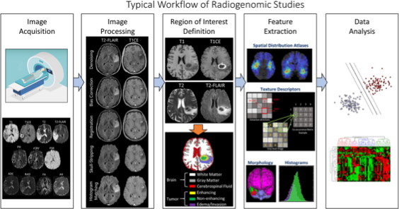
Typical workflow of radiogenomic studies[1]. 1) Image acquisition
2) Image processing, including noise/artifact reduction, intensity and/or orientation standardization, coregistration of the multiparametric MRI scans
3) ROI definition using manual annotation or automatic segmentation
4) Feature extraction based on human-engineered (conventional radiomics) or deep-learning approaches
5) Data analysis, involving machine/deep-learning methods for feature selection, classification, and cross-validation - Segmentation (U‑Net family)[2]
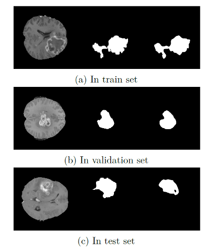
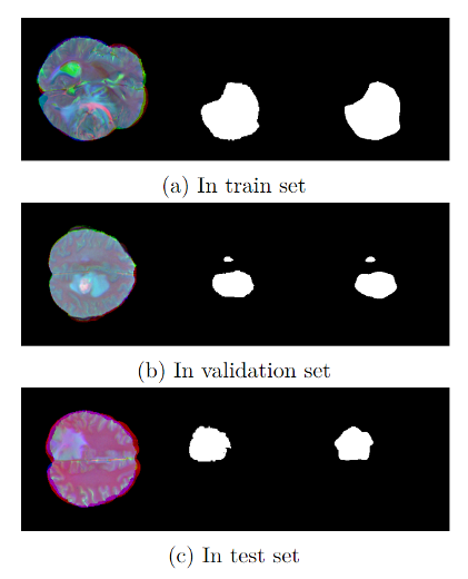
- Supervised learning with lesion masks; architectures based on U‑Net variants adapted for GBM MRI.
- Robust preprocessing and modality‑aware batching to handle sequence imbalance.
- Outputs include training dynamics and qualitative visualizations for each sequence.
- Architecture :
import torch from torch import nn class ConvBlock(nn.Module): def __init__(self, in_channels: int, out_channels: int, p: float = 0.3): super().__init__() self.net = nn.Sequential( nn.Conv2d(in_channels, out_channels, kernel_size=3, stride=1, padding=1, padding_mode="reflect", bias=False), nn.BatchNorm2d(out_channels), nn.Dropout2d(p), nn.LeakyReLU(inplace=True), nn.Conv2d(out_channels, out_channels, kernel_size=3, stride=1, padding=1, padding_mode="reflect", bias=False), nn.BatchNorm2d(out_channels), nn.Dropout2d(p), nn.LeakyReLU(inplace=True), ) def forward(self, x: torch.Tensor) -> torch.Tensor: return self.net(x)- Downsampling: strided 3×3 conv (stride=2).
- Upsampling: nearest‑neighbor upsample ×2 + 1×1 conv to halve channels; concatenate with encoder skip features.
- Depth: 64 → 128 → 256 → 512 → 1024 (encoder) with symmetric decoder.
- Output: 1‑channel mask with sigmoid activation.
- Key change: Dropout2d(p=0.3) in each ConvBlock improves generalization under limited data and reduces overfitting.
-
Down/Up sampling blocks and overall UNet:
import torch from torch import nn from torch.nn import functional as F class downSample(nn.Module): def __init__(self, channel: int): super().__init__() self.layer = nn.Sequential( nn.Conv2d(channel, channel, kernel_size=3, stride=2, padding=1, padding_mode="reflect", bias=False), nn.BatchNorm2d(channel), nn.LeakyReLU(inplace=True), ) def forward(self, x: torch.Tensor) -> torch.Tensor: return self.layer(x) class upSample(nn.Module): def __init__(self, channel: int): super().__init__() # reduce channels after upsample to match skip features self.layer = nn.Conv2d(channel, channel // 2, kernel_size=1, stride=1) def forward(self, x: torch.Tensor, skip: torch.Tensor) -> torch.Tensor: x = F.interpolate(x, scale_factor=2, mode="nearest") x = self.layer(x) return torch.cat((x, skip), dim=1) class UNet(nn.Module): def __init__(self, in_channels: int = 1, base: int = 64, p: float = 0.3): super().__init__() # Encoder self.c1 = ConvBlock(in_channels, base, p) self.d1 = downSample(base) self.c2 = ConvBlock(base, base * 2, p) self.d2 = downSample(base * 2) self.c3 = ConvBlock(base * 2, base * 4, p) self.d3 = downSample(base * 4) self.c4 = ConvBlock(base * 4, base * 8, p) self.d4 = downSample(base * 8) self.c5 = ConvBlock(base * 8, base * 16, p) # Decoder self.u1 = upSample(base * 16) self.c6 = ConvBlock(base * 16, base * 8, p) self.u2 = upSample(base * 8) self.c7 = ConvBlock(base * 8, base * 4, p) self.u3 = upSample(base * 4) self.c8 = ConvBlock(base * 4, base * 2, p) self.u4 = upSample(base * 2) self.c9 = ConvBlock(base * 2, base, p) # Head self.head = nn.Conv2d(base, 1, kernel_size=3, stride=1, padding=1) self.act = nn.Sigmoid() def forward(self, x: torch.Tensor) -> torch.Tensor: L1 = self.c1(x) L2 = self.c2(self.d1(L1)) L3 = self.c3(self.d2(L2)) L4 = self.c4(self.d3(L3)) L5 = self.c5(self.d4(L4)) R4 = self.c6(self.u1(L5, L4)) R3 = self.c7(self.u2(R4, L3)) R2 = self.c8(self.u3(R3, L2)) R1 = self.c9(self.u4(R2, L1)) return self.act(self.head(R1)) - Radiomics Feature Extraction
- Extract quantitative features from lesion ROIs using the PyRadiomics toolkit[3]; feature families cover intensity, texture, and shape.
- Subtype Classification
- Train a lightweight MLP on engineered radiomics features to predict GBM molecular subtypes.
- A baseline following prior work (Wang 2017) reaches ~92% accuracy on subtype prediction.
Results
T1 sequence
| Metric | Train | Validation | Test |
|---|---|---|---|
| Accuracy | 0.989330 | 0.987710 | 0.980175 |
| Balanced Accuracy | 0.920806 | 0.926565 | 0.785334 |
| Precision | 0.777257 | 0.712830 | 0.721325 |
| Sensitivity (Recall) | 0.848366 | 0.862156 | 0.577671 |
| Specificity | 0.993246 | 0.990973 | 0.992996 |
| F1‑score | 0.811257 | 0.780414 | 0.642738 |
| IoU | 0.682449 | 0.639901 | 0.473555 |
- Classification: an MLP on radiomic features achieves strong subtype discrimination (see repository for ROC/AUC details).
T2 sequence
| Metric | Train | Validation | Test |
|---|---|---|---|
| Accuracy | 0.989264 | 0.989870 | 0.984979 |
| Balanced Accuracy | 0.910587 | 0.909416 | 0.836919 |
| Precision | 0.789571 | 0.823274 | 0.803875 |
| Sensitivity (Recall) | 0.827365 | 0.824060 | 0.679117 |
| Specificity | 0.993809 | 0.994771 | 0.994722 |
| F1‑score | 0.808027 | 0.823667 | 0.736243 |
| IoU | 0.677890 | 0.700199 | 0.582589 |
FLAIR sequence
| Metric | Train | Validation | Test |
|---|---|---|---|
| Accuracy | 0.992049 | 0.992683 | 0.987521 |
| Balanced Accuracy | 0.927457 | 0.925201 | 0.852725 |
| Precision | 0.789571 | 0.823274 | 0.803875 |
| Sensitivity (Recall) | 0.859252 | 0.853861 | 0.709059 |
| Specificity | 0.996663 | 0.996541 | 0.996391 |
| F1‑score | 0.853110 | 0.862322 | 0.778177 |
| IoU | 0.741113 | 0.759359 | 0.636898 |
Stack sequence (multi-sequence stacked as RGB-like channels)
| Metric | Train | Validation | Test |
|---|---|---|---|
| Accuracy | 0.993412 | 0.993930 | 0.989395 |
| Balanced Accuracy | 0.946541 | 0.944896 | 0.797306 |
| Precision | 0.871109 | 0.881431 | 0.858787 |
| Sensitivity (Recall) | 0.896896 | 0.893092 | 0.785677 |
| Specificity | 0.996186 | 0.996700 | 0.995885 |
| F1‑score | 0.883814 | 0.887223 | 0.820607 |
| IoU | 0.791817 | 0.797306 | 0.695788 |
Across-sequence comparison (test set)
| Metric | T1 | T2 | FLAIR | Stack |
|---|---|---|---|---|
| Accuracy | 0.980175 | 0.984979 | 0.987521 | 0.989395 |
| Balanced Accuracy | 0.785334 | 0.836919 | 0.852725 | 0.797306 |
| Precision | 0.721325 | 0.803875 | 0.803875 | 0.858787 |
| Sensitivity (Recall) | 0.577671 | 0.679117 | 0.709059 | 0.785677 |
| Specificity | 0.992996 | 0.994722 | 0.996391 | 0.995885 |
| F1‑score | 0.642738 | 0.736243 | 0.778177 | 0.820607 |
| IoU | 0.473555 | 0.582589 | 0.636898 | 0.695788 |
Contributions
- We built and validated a GBM‑oriented, end‑to‑end radiogenomics pipeline: multi‑sequence lesion segmentation → ROI‑based radiomics extraction (PyRadiomics) → subtype classification.
Discussion
- Multi‑sequence fusion helps segmentation: stacking T1/T2/FLAIR as multi‑channel input improves boundaries and reduces false positives because each sequence contributes complementary contrast (T1 anatomical detail, T2 fluid/edema sensitivity, FLAIR CSF suppression highlighting peritumoral edema).
- Limitation (subtype labeling): a patient may express mixed molecular signatures. Our current pipeline assumes single‑label subtype per patient and cannot produce multi‑label predictions. A practical path is to adopt multi‑label learning (sigmoid outputs with thresholding), uncertainty‑aware calibration, or mixture‑of‑subtypes modeling to reflect heterogeneity.
- Concrete future directions:
1) 3D segmentation to derive volumetric (3D) radiomics features, potentially improving subtype discrimination over slice‑wise 2D features.
2) Move beyond hand‑crafted radiomics: explore end‑to‑end learning that maps images/ROIs directly to subtype, allowing the network to learn task‑specific representations.
Appendix
References
- Fathi Kazerooni, Anahita, et al. “Imaging Signatures of Glioblastoma Molecular Characteristics: A Radiogenomics Review.” Journal of Magnetic Resonance Imaging, 52(1), 2020, 54–69. DOI: 10.1002/jmri.26907.
- Ronneberger, O., Fischer, P., Brox, T. “U‑Net: Convolutional Networks for Biomedical Image Segmentation.” In: MICCAI 2015, LNCS 9351, pp. 234–241. DOI: 10.1007/978-3-319-24574-4_28.
- van Griethuysen, J. J. M., et al. “Computational Radiomics System to Decode the Radiographic Phenotype.” Cancer Research, 77(21), 2017, e104–e107. DOI: 10.1158/0008-5472.CAN-17-0339. (PyRadiomics)